您现在的位置：主页 > 上位机技术 > python > Python+Hadoop 从DBLP数据库中挖掘经常一起写作的合作者

本文所属标签:

Python+Hadoop 从DBLP数据库中挖掘经常一起写作的合作者

来源：网络整理网络用户发布，如有版权联系网管删除　2018-08-13　

本文的写作目的是从 DBLP 数据库中找到经常一起写作的合作者。熟悉数据挖掘中频繁项挖掘的经典算法( FP-Growth )并作出改进和优化。实验代码用Python写的，分别在本地(Win8)和Hadoop集群(条件有限，虚拟机上跑的，3个节点)上实现。(下载本文所涉及全部代码 https://github.com/findmyway/DBLP-Coauthor )

回复此公众号“ 作者 ”获取源码，以及word版原文查看。向小编咨询问题，联系微信:hai299014

首先从官网下载 DBLP 数据集只需下载 dblp.xml.gz 解压后得到 1G 多 dblp.xml 文件!文件略大。用 vim 打开文件后可以看到，所有的作者信息分布在以下这些属性中: 'article','inproceedings','proceedings','book','incollection','phdthesis','mastersthesis','www'

在这里使用 python 自带的 xml 分析器解析该文件(注意这里使用 sax 的方式)源码如下:(其核心思想为，分析器在进入上面那些属性中的某一个时，标记 flag=1 ，然后将 author 属性的内容输出到文件，退出时再标记 flag = 0, 最后得到 authors.txt 文件)

01 import codecs

02 from xml.sax import handler , make_parser

03 paper_tag = ( 'article' , 'inproceedings' , 'proceedings' , 'book' ,

04 'incollection' , 'phdthesis' , 'mastersthesis' , 'www' )

44 result . close ()

读取步骤 1 中得到的 authors.txt 文件，将其中不同的人名按照人名出现的次序编码，存储到文件 authors_index.txt 中，同时将编码后的合作者列表写入 authors_encoded.txt 文件。

02 source = codecs . open ( 'authors.txt' , 'r' , 'utf-8' )

03 result = codecs . open ( 'authors_encoded.txt' , 'w' , 'utf-8' )

04 index = codecs . open ( 'authors_index.txt' , 'w' , 'utf-8' )

05 index_dic = {}

06 name_id = 0

07 ## build an index_dic, key -> authorName value => [id, count]

08 for line in source :

09 name_list = line . split ( ',' )

10 for name in name_list :

11 if not ( name == ' rn ' ):

12 if name in index_dic :

13 index_dic [ name ][ 1 ] += 1

15 index_dic [ name ] = [ name_id , 1 ]

16 index . write ( name + u' rn ' )

18 result . write ( str ( index_dic [ name ][ 0 ]) + u',' )

19 result . write ( ' rn ' )

21 source . close ()

22 result . close ()

(这里注意编码，不然会出现UnicodeError，很蛋疼的。。。)

查看在 DBLP 数据集中作者发表文章的数量。即统计只发表过 1 次文章的人数有多少，发表过 2 篇文章的人数有多少 ...... 发表过 n 篇文章的有多少人 ... 并且绘图:

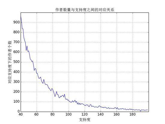
分析可知，当支持度为 40 的作者数量接近 1000 ，随后支持度每增加 20 ，对应的作者数量减半，为了降低计算量，第一次实验时支持度阈值不宜选得太小，同时为了避免结果数量太少，初次实验时阈值可选在 40~60 之间(在接下来的实验中选的是 40)。

view_data.py

01 from matplotlib.font_manager import FontProperties

02 font = FontProperties ( fname = r"c:windowsfontssimsun.ttc" , size = 14 )

04 import matplotlib.pyplot as plt

05 import numpy as np

06 data = codecs . open ( 'authors_encoded.txt' , 'r' , 'utf-8' )

07 word_counts = {}

09 for line in data :

10 line = line . split ( ',' )

11 for word in line [ 0 : - 1 ]:

12 word_counts [ word ] = word_counts . get ( word , 0 ) + 1

13 if word_counts [ word ] > maxCounts :

14 maxCounts = word_counts [ word ]

17 xMax = maxCounts

18 data . close ()

20 for k , v in word_counts . iteritems ():

21 bins [ v ] = bins . get ( v , 0 ) + 1

23 for i in range ( 40 , 200 ):

24 y . append ( bins . get ( i , 0 ))

25 plt . plot ( y , '-' );

27 plt . yticks ( range ( 0 , 1000 , 100 ))

28 plt . xticks ( range ( 0 , 160 , 20 ), range ( 40 , 200 , 20 ))

29 plt . xlabel ( u'支持度' , fontproperties = font )

30 plt . ylabel ( u'对应支持度下的作者个数' , fontproperties = font )

31 plt . title ( u'作者数量与支持度之间的对应关系' , fontproperties = font )

构建 FP-Tree 并从 FP-Tree 得到频繁项集

FP-Tree 算法的原理在这里不展开讲了，其核心思想分为 2 步，首先扫描数据库得到 FP-Tree, 然后再从树上递归生成条件模式树并上溯找到频繁项集。这里借用 Machine Learning in Action 中的核心代码。(写得真心好，值得深入学习)。

157 ConA , ConB , ConC , MinCon , MaxCon ))

在选取频繁度为 40 后发现，得到的结果非常多，总共 2000 多，为了分析的方便，进一步提高频繁度阈值为 100 ，此时得到了 111 条记录，按照合作者的共同支持度排序，部分截图如下:

再对该结果文件分析发现，输出结果降低到 82 条，同时可以看到 MinCon 分布在( 0.3,0.4 )之间的记录很少，因此，可以考虑将 MinCon 的阈值调整到 0.4

在这里将作者与其合作者之间的关系用图来表示以排名在最前面的作者 Irith Pomeranz 为例.

并行 FP-Growth 算法最早研究可以参考文献:

Parallel_Frequent_Pattern_Mining.pdf

并行 FP-growth 算法可分解为两个 MapReduce 过程。

第一轮 MapReduce 所做的工作就是一个 WordCount ，扫描整个数据，统计每个词项所出现的次数。具体说来就是在 Map 过程中，输出以下键值对 <word, 1> ，在 Reduce 过程中，统计 word 出现的总的次数。具体可参考:

第二轮 MapReduce 过程是并行 FP-growth 算法的核心。

1. 读取第一轮 MapReduce 所得到的的词频，得到一个词典的数据结构;

2. 依次从数据库读取记录，并根据上一步中的词典结构对其排序，同时过滤掉不满足支持度阈值的词项;

3. 输出排序后记录中每一个元素的条件模式项，具体为什么这么做可以回顾 FP-growth 算法的原理

1. 获取每个元素所对应的条件模式项，并统计条件模式项中每个词项出现的次数

2. 对条件模式项中的每个词频用支持度阈值过滤

3. 从该条件模式项中生成其所有子集即为最后的结果(这一步在上图中没有，我自己加进去的)

Hadoop 平台上实现 FP-Growth 算法

理解上面的算法原理后，实现起来就比较容易了。

第一轮的 MapReduce 可以参考: www.tianjun.ml/essays/19

01 #!/usr/bin/env python

03 def creatDic ():

04 freqDic = {}

05 with open ( 'sortedList' , 'r' ) as sortedList :

06 for line in sortedList :

07 line = line . strip () . split ( ' t ' )

08 freqDic [ int ( line [ 0 ])] = int ( line [ 1 ])

09 return freqDic

11 def read_input ( inFile ):

12 for line in inFile :

13 yield line . split ( ',' )

15 def main ( freqDic , minSup ):

16 data = read_input ( sys . stdin )

17 for names in data :

18 names = { name : freqDic [ int ( name )] for name in names

19 if name . isdigit ()

20 and freqDic . get ( int ( name ), 0 ) >= minSup }

21 lenth = len ( names )

22 if lenth >= 2 :

23 conPatItems = [ name for name , value in

24 sorted ( names . iteritems (),

25 key = lambda p : p [ 1 ])]

26 for i in range ( lenth - 1 ):

27 print " %s t %s " % ( conPatItems [ i ], conPatItems [ i + 1 ::])

31 if name == ' main ' :

33 dic = creatDic ()

02 from itertools import groupby

03 from operator import itemgetter

06 def readMapOutput ( file ):

07 for line in file :

08 yield line . strip () . split ( ' t ' )

10 def main ( minSup ):

11 data = readMapOutput ( sys . stdin )

12 for currentName , group in groupby ( data , itemgetter ( 0 )):

15 for currentName , conPatItems in group :

16 conPatItems = conPatItems . strip () . strip ( '[' ) . strip ( ']' )

17 #print "%st%s" % (currentName, conPatItems)

18 itemList = conPatItems . split ( ',' )

19 for item in itemList :

20 item = item . strip () . strip ( "'" )

21 item = int ( item )

22 localDic [ item ] = localDic . get ( item , 0 ) + 1

23 resultDic = { k : v for k , v in localDic . iteritems ()

24 if v >= minSup }

25 #Here we just print out 2-coauthors

26 if len ( resultDic ) >= 1 :

27 print " %s t %s " % ( currentName , resultDic . items ())

30 print " %s t %s " % ( "inner err" , "sorry!" )

33 if name == " main " :

本次实验分别在本地和Hadoop集群上实现了DBLP数据集中的合作者挖掘，由于实验条件有限，Hadoop集群为虚拟机实现，故难以对本地单机运行效率和分布式运行的效率进行对比，不过从论文 Parallel_Frequent_Pattern_Mining.pdf 的分析结果可以看出，在数据量较大的时候分布式运行的FP-growth算法要比常规的FP-growth算法运行效率高很多。

不得不说，MapReduce的调试要比普通程序的调试要复杂的多，一个建议是先将Reduce的任务设为0，查看Map输出是否是想要的结果，或者直接在Reduce过程中打印出收到的整理后的Map输出，方便进一步分析。

写程序的过程中出了个很蛋疼问题，分布式的输出和单机模式下的输出结果不同!!!找了半天才发现分布式的输出结果因为没有挖掘完整的频繁项，比如输出的<key, value>中 value 为<authorA,authorB,authorC>的话，并没有输出其子集<authorA,authorB> <authorA,authorC>和<authorB,authorC>以至分布式下的输出结果比单机下的结果数量要少。

最后的最后，不得不吐槽下编码以及字符串的处理......

via:http://www.tianjun.me/essays/20/

　　　　　　　　　　　　　查看评论回复

嵌入式交流网主页 > 上位机技术 > python > Python+Hadoop 从DBLP数据库中挖掘经常一起写作的合作者

输出结果作者